
Hello Jax
JAX is quickly becoming a popular framework for training Deep Learning models. I
spent some time playing around with it last year, so decided to share some basic
stuff that I learnt in case someone finds it useful. This tutorial implements
logistic regression with Autograd in JAX.
At its core, JAX is essentially a numerical computation library, like Numpy but
with support for accelerators like GPU and TPU, and with a robust support for
differentiation (Autograd). In this tutorial, we’ll be implementing a logistic
regression from scratch in JAX to give a very basic introduction to JAX. The GIF
below shows what we’ll be implementing today.
This tutorial is also available as a Google Colab here
Setting Up
We start by importing some common modules. Note that JAX has it’s own
implementation of numpy, which we commonly import as jnp to avoid confusing
with the default numpy implementation, which is usually imported as np.
import jax
from jax import grad, numpy as jnp

import glob
import imageio
import matplotlib.pyplot as plt
Next we generate a toy dataset to run logistic regression on. We start by generating a PRNG key. This is one of the interesting differences between JAX and other frameworks: JAX explicitly requires passing a PRNG key every time to generate random numbers. One gotcha here is that if random number generation is called with the same PRNG key, the same set of numbers is returned. The recommended way to generate new random numbers is to split they key
key = jax.random.PRNGKey(0)
# Generating a toy dataset of 500 points and 2-dimensional data between -1 to 1.
x = jax.random.uniform(key, shape=[500,2], minval=-1.0, maxval=1.0)
# Setting a linear decision boundary for creating labels.
t = 0.5*x[:,0] + 0.75*x[:, 1] -0.3
# Creating labels based on the linear boundary.
y = (t>0).astype(float)
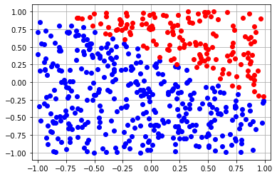
We add a helper method to plot points and visualize the dataset.
def plot_points(x, y, params=None):
  positive_labels = x[jnp.where(y==0.0)[0]]
  negative_labels = x[jnp.where(y==1.0)[0]]
  plt.plot(positive_labels[:, 0], positive_labels[:, 1], 'bo')
  plt.plot(negative_labels[:, 0], negative_labels[:, 1], 'ro')
  plt.xlim([-1.05,1.05])
  plt.ylim([-1.1,1.1])
  if params:
    x_range = jnp.linspace(-1.0, 1.0, 100)
    y_boundary = -params[1]/params[0][1] - params[0][0]*x_range/params[0][1]
    plt.plot(x_range, y_boundary, 'g-', linewidth='3')
  plt.grid()

plot_points(x, y)
This should generate the following plot:
Defining the Model
In this section, we define the model, loss function and verify that gradient calculation is working as expected. The model is a simple logistic regression model, so the model looks like:
\[h_i = \sigma(w^Tx_i + b)\]and the loss function is the standard binary cross-entropy loss:
\[loss = -\sum_i y_i log(h_i) + (1-y_i)log (1-h_i)\]We start by defining the params for our
model. Since the data is 2-dimensional, we need to define two params, the weight
vector \(w\), and the bias term \(b\). Another interesting thing is that even if
params are a nested list or dictionary, Autograd would still work fine.
w = jax.random.uniform(key, shape=[2,1])
b = jax.random.uniform(key, shape=[1,])
params = [w, b]
print(params)
Next we define the model and the loss function:
def h_theta(params, x):
  h = x@params[0] + params[1]
  h = jax.nn.sigmoid(h)
  return h

def loss(params, x, y):
  h = h_theta(params, x)
  h = jnp.reshape(h, [-1,])
  log_h = jnp.log(h)
  inv_log_h = jnp.log(1-h)
  return -jnp.sum(log_h*y + inv_log_h*(1-y))
The simplest way gradient calculation works in JAX is by calling the grad
method on any function. By default, the gradient is calculated w.r.t the first
parameter of the method. For example, for a function loss(params, x, y),
grad(loss) would return a function that calculates the gradient of the method
loss at (params, x, y) w.r.t params. To make sure gradient calculation is
working as expected, we can calculate the gradient manually as well.
Vectorially, this can be represented as \(\frac{\partial loss}{\partial w} = x^T(h-y), \frac{\partial loss}{\partial b} = (h-y)\)
\[\nabla_\theta loss = \begin{bmatrix} \frac{\partial loss}{\partial w} \\ \\ \frac{\partial loss}{\partial b} \end{bmatrix} = \begin{bmatrix} x^T(h-y) \\ \\ h-y \end{bmatrix}\]We can verify this in JAX with the following code:
# Calculating gradient with Autograd.
g = grad(loss)(params, x, y)
print(g)

# Calculating gradient manually.
ht = h_theta(params, x)
ht_y = (ht - jnp.reshape(y, [-1,1]))
print(jnp.transpose(x) @ ht_y)
print(jnp.sum(ht_y))
The two gradients calculated should match exactly. Finally, we are ready to run gradient descent.
Running Gradient Descent
If you’re running this in Colab, we create a new directory to store images of how the decision boundary changes after every step of gradient descent.
!mkdir /content/images
To run gradient descent, we set a learning rate of 0.01 and use the standard update rule for gradient descent.
alpha = 0.01
loss_values = []

for i in range(20):
  plot_points(x, y, params)
  plt.savefig('/content/images/%03d.png'%i)
  plt.show()
  grads = grad(loss)(params, x, y)
  params[0] -= alpha * grads[0]
  params[1] -= alpha * grads[1]
  l = loss(params, x, y)
  loss_values.append(l)
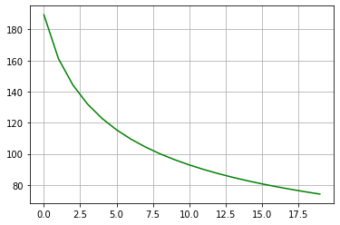
We can plot the loss_values to see how they change with each step.
loss_values = [float(i) for i in loss_values]
plt.plot(range(len(loss_values)), loss_values, 'g-')
plt.grid()
This is what the plot should like:
To generate a GIF of how the decision boundary changes with each step, we can run the following code in Colab:
fileList = glob.glob('/content/images/*.png')
fileList.sort()

with imageio.get_writer('/content/grad_descent.gif', mode='I') as writer:
    for filename in fileList:
        image = imageio.imread(filename)
        writer.append_data(image)
This should generate the following plot: